In excel, names can refer to cells, a specific value or a formula. These names can be used to make complex formulas easy to read and understand as you refer to the names instead of using a constant value or cell reference. The names can also serve as a data source in a data validation drop down list.
One key reason for using names in modelling is to ease the model audit process. The modeler can define cells used in formulas to make it easy for the model auditor to understand the workings of the model. Doing this could save a lot of back and forth between the modeler and the model auditor.
Now that we have established how important names are in excel and some of the uses of names, let's show you how to create and use names in excel.
There are 3 ways to define a name in excel: these are through the name box, define name box and through the Excel name manager. Let's treat each method below:
Through the name box
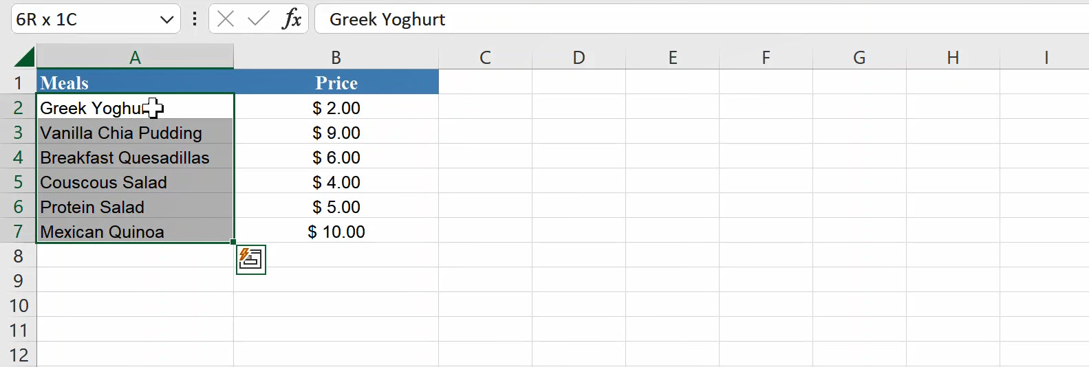
This method is the easiest and fastest way to define names for a range of cells in excel. There are basically just 3 steps involved. The first step is to select the cell or range of cell you want to define.
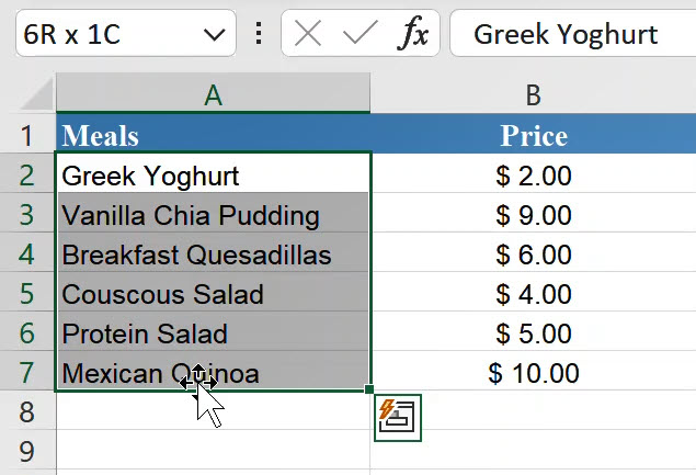
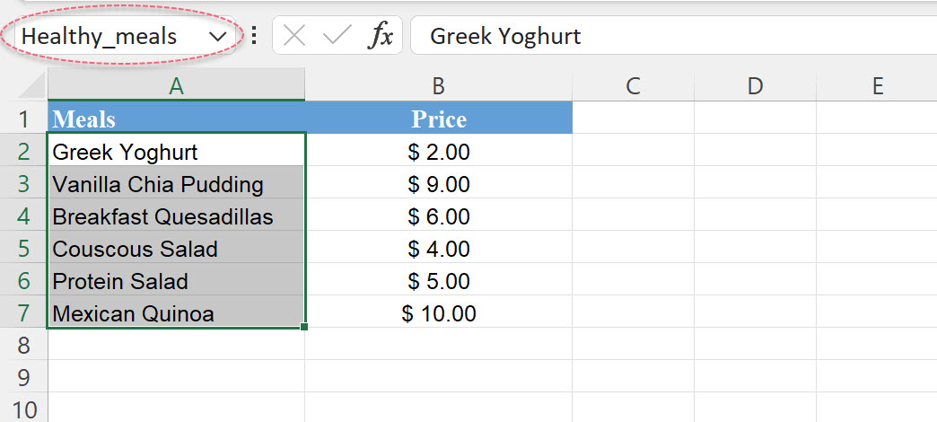
Step 2: Navigate to the name box and type in a name. In our example we want to define this range as healthy meals
Step 3: Press Enter
Through the Define Name Button
This section takes you through the steps for defining names through the name button in the formula tab. Let's begin.
Step 1: Select the cells you want to define, like we did in the previous section.
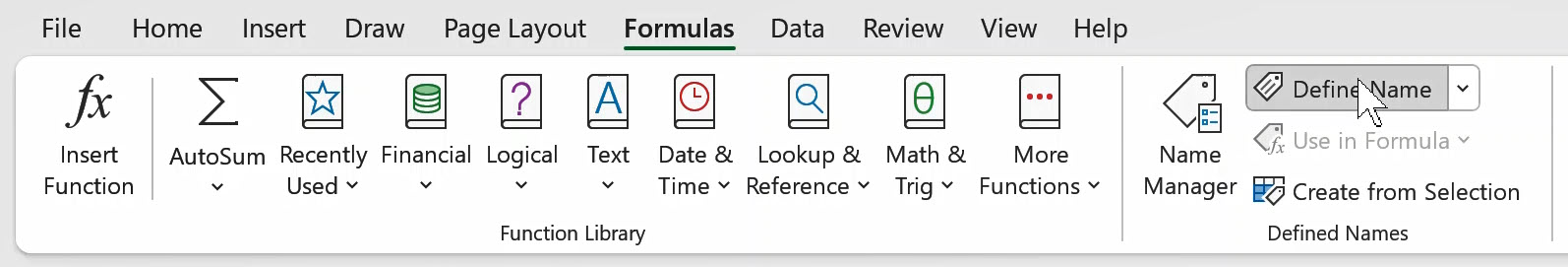
Step 2: Navigate to the formula tab > Define Names Group > Define Names button
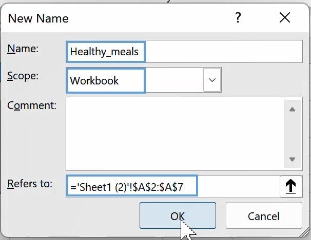
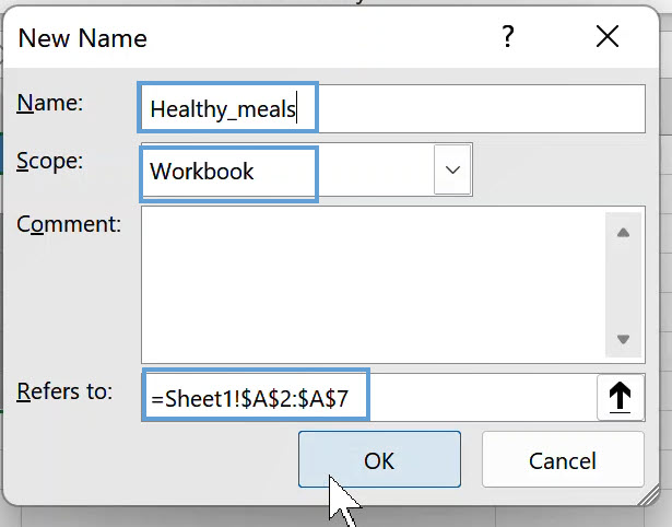
Step 3: In the new name dialog box, specify the following:
- Type in the name you want to assign to the cell(s) selected in step 1, note that you would need to use underscores to connect two or more word names.
- Scope: The default is the entire workbook, but you can limit it to a particular worksheet by using the dropdown
- Finally, double check that the refers to box is referring to the correct cells, otherwise make adjustments accordingly.
Through the Excel Name Manager
The last method we would be touching on for defining names in Excel is through the Excel name manager. Let's show you how to go about it:
Step 1: Select the cell(s) you want to define.

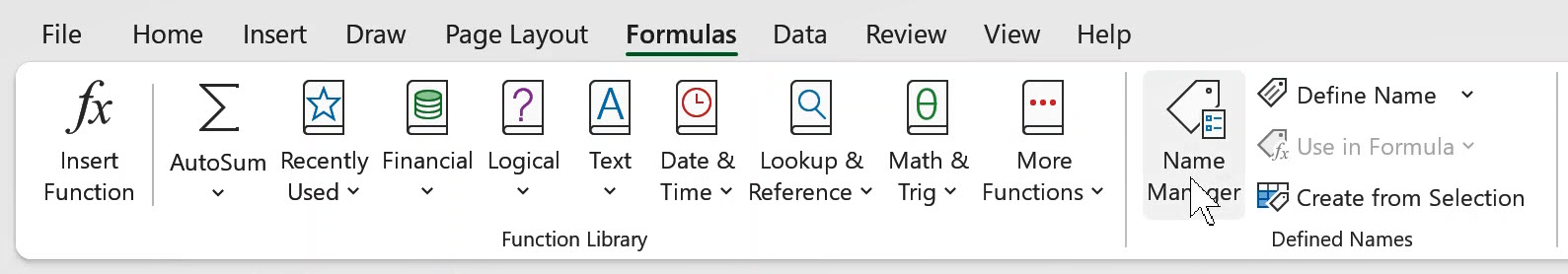
Step 2: Navigate to the formula tab > Define Names Group > Name Manager
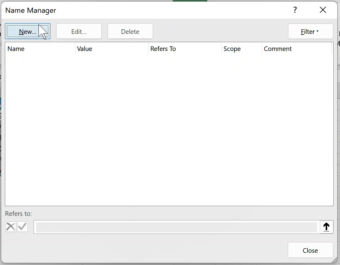
Step 3: Click on new at the top left corner of the name dialog window.
Step 4: Attend to the highlighted categories as discussed in the define name button section and click OK.
Operations with Named Ranges
In this section we would take you through how you can apply named ranges to your calculations in excel. Let's start with naming a constant and referring to the name in your formula
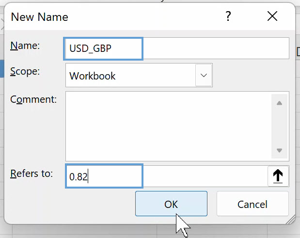
Create Excel name for a Constant
Using our same example, let's assume we are moving to a new market (specifically the UK market), we would need to convert the prices of our products to the British Pound. To do this we can define a constant (GBP multiplier) to apply across the product rows for conversion.
Step 1: Navigate to the Name Manager using the guides in the previous section and define a GBP multiplier
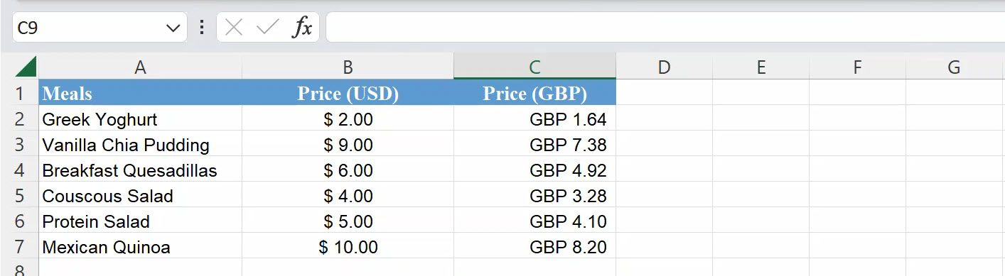
Step 2: Apply the new name to your multiplication formula as seen below
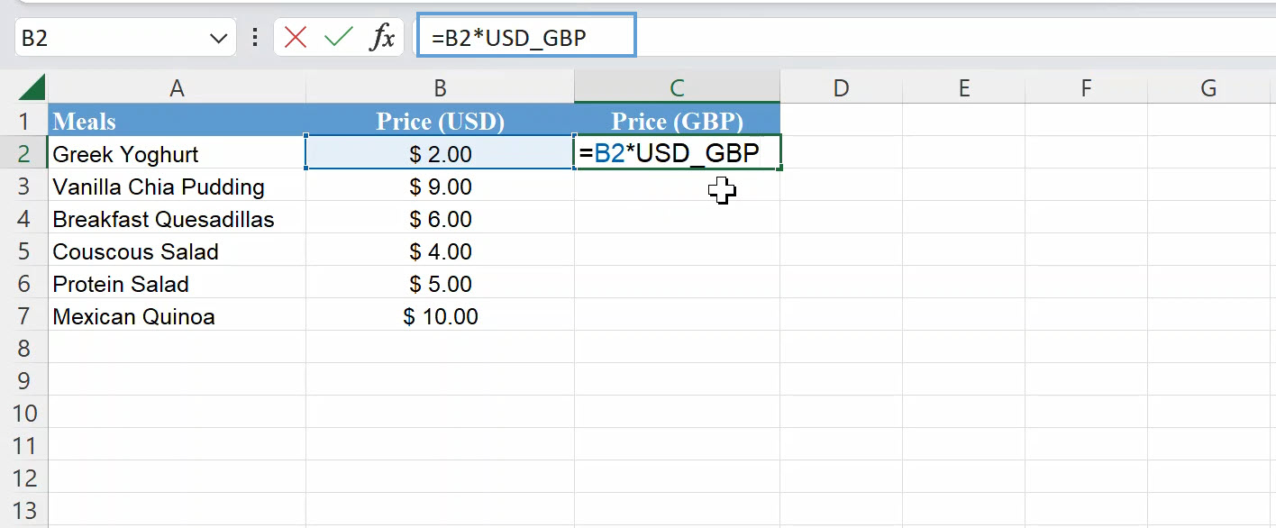
Step 3: Drag the formula to the rows below or Copy and Paste using Ctrl + C and Ctrl + V
Define Names for a Formula
In this section, we would be counting the number of meal offerings by using =defined name. First let's define a name for a Count Formula. The count formula we would be treating counts the number of non-blank cells in the range specified.
Step 1: Open up the name Manager using the steps we treated in the previous section
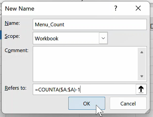
Step 2:
- Assign an easy to remember name in the name box
- In the refers to box, type in =COUNTA($A:$A)-1
Note: The minus one ("-1") at the end of the formula is to remove the heading in cell A1 so that we have a true count of our menu
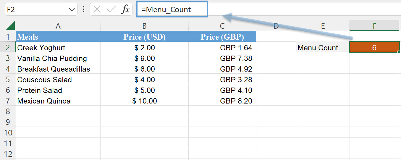
Step 3: Type in the formula =Menu_Count and press Enter
Create a Dynamic Named Range
In this section, we would show you how to create a dynamic named range, that is a range that automatically adjusts depending on data provided. To Illustrate, we would continue with the same data set of healthy meals we have stuck to since the beginning of this post. Our task now is to add up the total cost of all our meal offerings assuming a customer walks in and decides to purchase all our products. But remember, we may add new products in future, so we want a formula that automatically updates when we add new products.
To accomplish the above task, we would need to combine some functions such as the Offset and CountA functions. Let's see the steps in detail below:
Step 1: Open up the name manager as discussed in previous sections
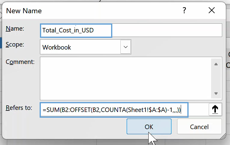
Step 2:
- In the name box, assign a name to the new function we are looking to create
- In the refers to box, type in the following formula below and click on OK once done
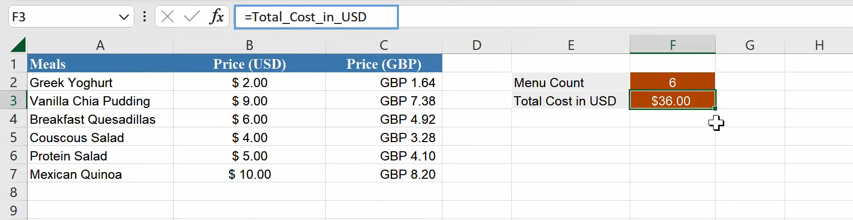
Step 3: Navigate to the cell you have designated to calculate the sum of all the products in USD and simply type in =Total_Cost_in_USD
Breaking down the formula
Sum Function: This is pretty straightforward, just adding up the data within a range, i.e from starting point B2 to an end point we would specify with a combination of the Offset and CountA functions.
Offset Function: The Offset function returns a range of cells. In the formula you specify an initial cell (which is B2 in our case), then you specify the number of columns and rows to move for excel to arrive at a new cell. In our formula our initial range is cell B2, and we want to arrive at cell B7 to complete the range in our sum formula above. We however don't want to manually specify that excel should go down 6 rows from our starting point because we want the number of rows to be dependent on the menu we have. To achieve this, we employ the use of the CountA function for the row number.
CountA function: The count A function counts cells containing any and every type of information within the range you specify. Meaning that as far as the cell is not blank, excel would count it. This function within our formula is used to specify the number of rows excel should pick for our Offset Formula. This is a key part to what makes the formula dynamic as the number of rows for our offset function changes when we add more meals to column A.
Testing all we've done
Let's add a new item to the menu and see if our count and total cost would be updated.
If you need to practice all we have discussed in this post, please download the template below. Hope to see you in other posts, bye.