Table of Contents[Hide][Show]
Adding a filter to a dataset is easy to do when your data is uniform. However, when there are empty rows within the data, it becomes a little challenging. This is because excel cuts off data appearing after the empty rows. In today's post we would take you through a quick hack to circumvent this.
First: Prepare your Data
Preparing your data is not as difficult as it sounds. Infact, it is super easy, barely an inconvenience (if you know, you know). All you need to do is to select the complete data. Take for example the summary financials & ratio data we have prepared below.
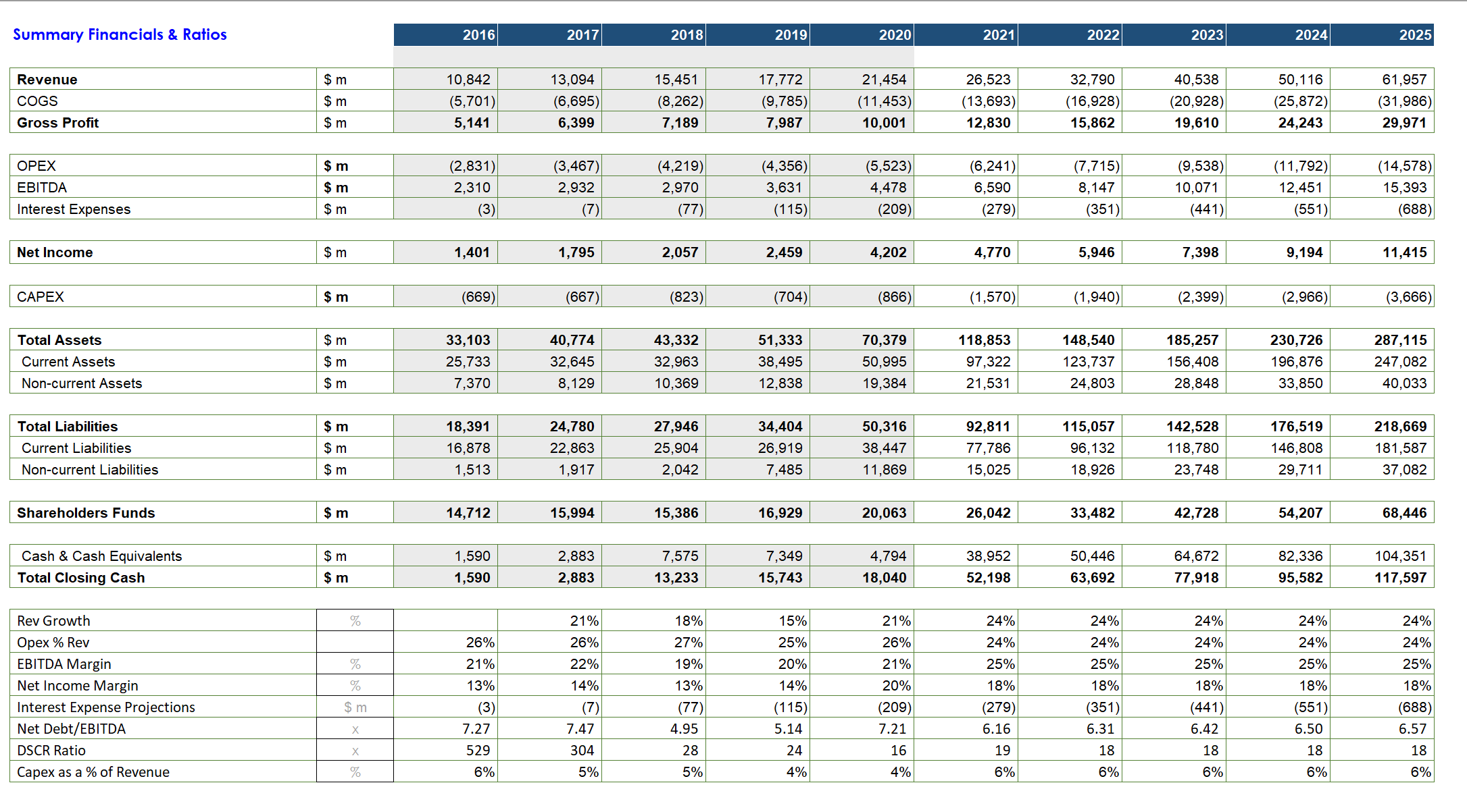
For presentation purposes we have included some rows in between major headings, however when reviewing we might need to compare some headings to see if things add up. For instance we need only 3 headings to be displayed one row after another. These headings are Total Assets, Total Liabilities and Shareholders Funds. We can achieve this through filtering our data, but we need to select the whole data first.

Apply the Filter
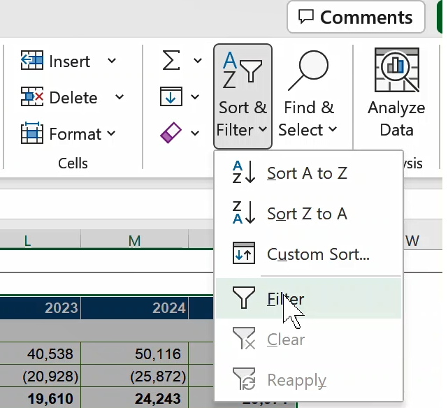
Step 1: Whilst still selecting the data, navigate to the home tab and in the Editing group, click on Sort & Filter.
Step 2: Excel automatically adds the filter cone to the first row of the data you have selected.
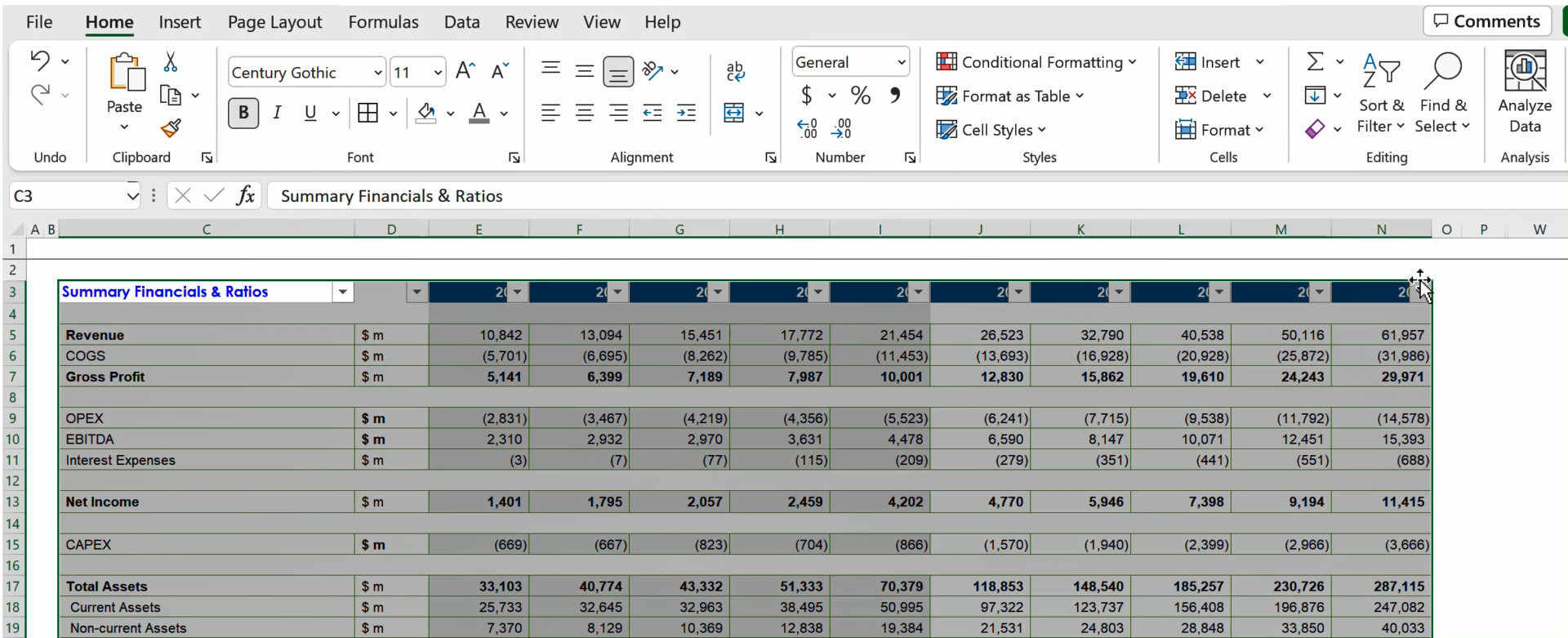
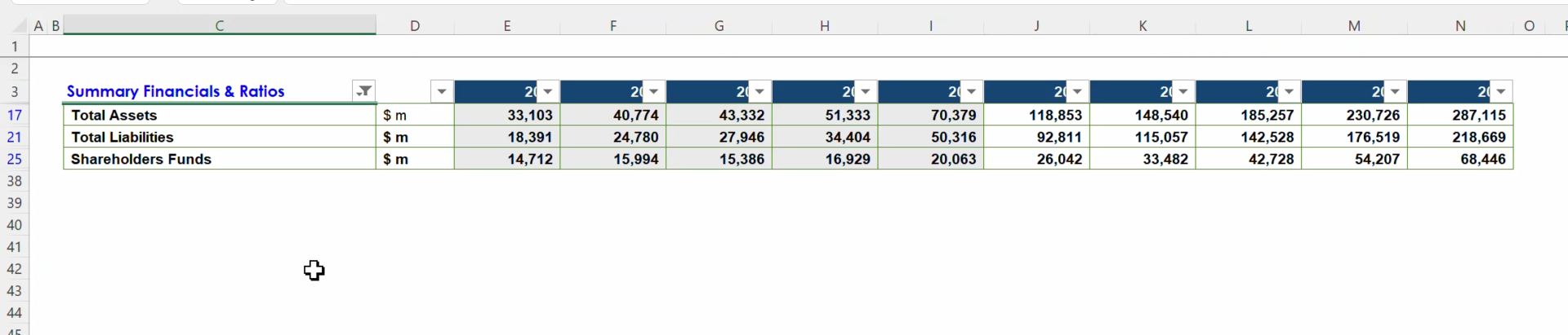
Now we can filter for Total Assets, Total Liabilities and Shareholders funds in Cell D3

Result: Now we have the 3 headings stacked on top of the other
All done, remember to use this anytime you need to filter data with some blank rows in it. See you in another post, bye.