The first step in adding filter options to every column in an Excel pivot table is to create the pivot table from your dataset. Ensure the pivot table is set to a compact layout for a clear display after your data fields have been organized in the Rows and Columns sections.
Turn on the "Field Headers" option. This one is usually located under the "Report Layout" settings under the "Design" tab. This is an important step since it allows each column to have its own set of filter options.
Choose any cell in the pivot table after ensuring all the parameters are correct. A drop-down arrow in each column header shows the availability of filter choices. You can filter each column according to particular standards by clicking on these drop-down arrows.
By carefully filtering each column in the pivot table, this method allows users to customize their data analysis. The additional filter options improve the interactive features of the pivot table, making it easier to explore and analyze data effectively, regardless of the requirement to concentrate on particular categories, periods, or other aspects. By allowing users to swiftly filter data across all columns, this straightforward yet effective tool guarantees that users can immediately improve their insights, resulting in a more efficient and tailored Analysis.
Overview of Steps
In an Excel pivot table, adding filters to every column entails turning on the "Field Headers" option to enable separate filters for every column. Here's a quick rundown of the steps (don't worry, we would have a visual representation in our examples section):
- Choose Pivot Table: Launch the pivot table and click on any cell to get started. This guarantees that the pivot table you wish to change will be the center of your attention.
- Select the "Design" tab on the Ribbon to activate the field headers. Verify that the "Field Headers" option is enabled under the "Design" tab. To enable filter options in each column, follow this key step.
- Find the "Report Layout" settings under the "Design" tab to display in compact form. Select the option "Show in Compact Form" from the menu. In addition to displaying a drop-down arrow for each column, this action activates the "Field Headers".
- Use Filter Drop-down Arrows: When "Field Headers" is turned on, a drop-down arrow will appear in the header of each pivot table column. To view the filter choices for a given column, click the arrow located in the column header.
- Apply Filters: You can select particular things to include or omit from the column using the filter's options. Additionally, you can sort, filter based on criteria, or remove a column's filter.
Following these steps, you can tailor data analysis based on particular criteria by enabling filter options for each column in your pivot table. There is no special syntax or parameter needed for this simple process.
Usage Note
An Excel pivot table's ability to customize and analyze data is improved by adding filters to each column. To ensure a smooth experience, refer to these usage notes:
- Activate Field Headers: Ensure "Field Headers" are turned on before adding filters. This is located under the "Design" tab. To enable filter choices in every column, you must activate this option.
- Compact Form Layout: Select a "Compact Form" layout from the "Design" tab's "Report Layout" menu. To enable for customized filters, this step activates the "Field Headers" and shows a drop-down arrow for each column.
- One Click for Filters: To modify the pivot table, click on any cell. This guarantees that operations you perform on the pivot table, like adding filters, will be applied to the whole thing.
- Make Use of Drop-down Arrows: The header of every column now has a drop-down arrow. To view the filter choices for the appropriate column, click on these arrows. This makes precise and personalized filtering possible.
- Customization of Individual Columns: Filter can be applied separately to every column based on predetermined standards. Users can add or remove items, sort the data, or apply conditional filters to customize the analysis to their needs.
- Several Filter Combinations: Make use of the opportunity to apply filters to several columns at once. This makes it possible to combine complicated filters, which improves analysis and yields more specific insights from the data.
- Dynamic Data Exploration: Data can be dynamically explored using filters. Users may quickly switch between filters with only a few clicks, changing the pivot table's look to highlight various dataset features.
- Unmistakable Visual Cue: The drop-down arrows clearly show which columns currently use filters. This clarity improves the general user experience and comprehension of the applied filters.
- Maintaining Uniformity Throughout Worksheets: Ensure the filters are applied consistently if your worksheet has several pivot tables. This guarantees that the same standards are applied to all data representations.
- Record Filtering Criteria: You should think about recording the filtering criteria used for each column for future use or collaborative effort. This procedure guarantees openness and aids in preserving analysis clarity.
Examples on Adding Filter to Columns in Pivot Tables
Product Sales Analysis
In our example, we have a data set with product names, region and sales performance. We would use this data set to take you through how to add filter to the columns. Our pivot table will summarize the information by product name.
To apply filters to every column, we only need to follow these simple steps
- Create a PivotTable with "Product Name," "Region," and "Sales" fields. Drag "Product Name" to Rows, "Region" to Columns, and "Sales" to Values (Sum).
- Click the arrow next to any "Product Name" in the rows area.
- A list of all products will appear.
- Check/uncheck the products you want to include/exclude.
- Click "OK" to apply the filter.
- Click the arrow next to any "Region" header.
- A list of all regions will appear.
- Check/uncheck the regions you want to include/exclude.
- Click "OK" to apply the filter.
Time-Based Revenue Analysis
Consider a pivot table with columns for the years, quarters, and revenue that shows revenue data Ensure your data includes columns for "Year," "Quarter," and "Revenue.". To include filters to your data set, just follow these simple steps:
- Create a PivotTable:
- Select any cell in your data range.
- Go to Insert > PivotTable.
- Choose a new worksheet or existing location.
- Drag "Year" to the Rows area.
- Drag "Quarter" to the Columns area.
- Drag "Revenue" to the Values area (choose "Sum").
- Click the down arrow next to any year in the Rows area.
- A list of all years appears.
- Check/uncheck the years you want to include/exclude.
- Click OK to apply the filter.
- Click the down arrow next to any quarter header in the Columns area.
- A list of all quarters appears.
- Check/uncheck the quarters you want to include/exclude.
- Click OK to apply the filter.
Employee Performance Metrics
Let's say you have a pivot table containing columns for employee name, department, performance score, and other employee performance measures. This is how filters are added:
- Make sure your data includes columns like "Employee Name," "Department," "Performance Score," and other relevant performance metrics.
- Select any cell within your data range.
- Go to the Insert tab and click PivotTable.
- Choose to create a new sheet or place it on your existing sheet.
- Drag "Employee Name" (optional) to the Rows area.
- Drag "Department" to the Filters area and keep it unchecked (to show all departments).
- Drag "Performance Score" and other metrics to the Values area, choosing "Sum," "Average," or other desired calculations.
- Click the arrow next to the Department field in the Filters area.
- A list of all departments will appear.
- Check the boxes next to the departments you want to include.
- Uncheck the box next to "Select All" if you don't want to show all departments.
- Click OK to apply the filter.
Uses of Filter Option for Columns in Pivot Tables
There are many advantages to adding filters to Excel pivot table columns, allowing users to personalize their data analysis. The following are the main applications for which adding filters to pivot table columns is useful:
- Filters allow users to focus on particular categories, periods, or other criteria while viewing data in each column. To obtain focused insights, this selective observation is essential.
- Accurate Data Interpretation: By using filters on certain columns, users may accurately interpret data. When analyzing particular characteristics or dimensions inside a dataset, this is extremely helpful.
- Data Exploration that is Dynamic: Using filters allows for dynamic data exploration. With the ability to quickly and interactively explore data, users can quickly switch the pivot table view by toggling filters on and off.
- Individualized Data Presentations: Adding filters can make data presentations according to specific requirements. Users can customize the pivot table to highlight particular data pertinent to their analysis or presentation needs.
- Comparative Analysis: By enabling users to concentrate on subsets of data within various columns, filters help with comparative studies. Finding trends, patterns, or differences between categories can benefit from this.
- Time-Based Analysis: Filters on columns allow you to concentrate on particular periods when working with time-based data, which makes it easier to do trend analysis, identify seasonal patterns, and compare data from year to year.
- Data segmentation is made possible via filters, which let users look at subsets of information according to parameters like product categories, client segments, or geographical areas.
- Effective Report Creation: Filters improve report creation effectiveness by allowing users to see particular data points without requiring a lot of manual sorting or pivot table rearranging.
- The addition of filters facilitates drill-down analysis. By drilling down into certain elements inside columns, users can gain more detailed insights after beginning with a high-level overview.
- Clarity in Visual Indications: Filters make the criteria applied to each column evident. Because all stakeholders are aware of the context of the data, this transparency fosters better collaboration and communication.
- Filters enable the examination of data on the spot. To explore various aspects of the data with flexibility, users can swiftly modify the filters in response to changing analytical requirements.
- Users gain the ability to perform targeted, dynamic, and personalized data analysis by adding filters to columns in pivot tables, which improves process efficiency and insight.