The excel INDEX function is used to return a value at a given location in a range or array. The User could specify the row and column number manually, and through combination with other functions such as MATCH Function, the row number or column number can be automatically calculated based on single or multiple criteria. The INDEX can extract individual values, entire rows and columns. In today's post, we would take you through all you need to know about the INDEX function. Let's begin with the syntax and argument.
Syntax & Argument
The syntax of the INDEX Function is as follows:
=INDEX(array, row_num, [col_num], [area_num])
- Array (required): Range or array to retrieve the values you desire. If you choose not to specify the column number, this is the exact column where the value you desire can be found (A1:A15). If however you decide to specify the column number, then you would need to select the complete data set (A1:E15)
- row_num (required if col_num is omitted): Represents row number in the array from which to retrieve a value.
- Col_num (required if row_num is omitted): Represents column number in the array from which to retrieve a value.
- [area_num] (optional): This is an optional parameter that specifies which range from the reference argument to use. This is only valid when you specify 2 or more ranges in the array argument.
Things to note
- If rows are omitted and columns supplied manually, the INDEX Function retrieves data of entire rows for the columns specified.
- If columns are omitted and rows supplied manually, the INDEX Function retrieves data of entire columns for the rows specified.
- If both rows and columns are omitted, the INDEX function retrieves the range specified in the array argument or retrieves the area specified if area_num argument is provided.
Now let's see some examples below:
INDEX Function Examples
The INDEX function syntax varies depending on how the user applies it. The user could set the range to be one dimensional (data set formatted into a single column or single row) or set the range to be two dimensional. As discussed in the previous section under syntax, the row and column numbers could be either required or optional arguments depending on the data dimensions or intent of the user. Let's move to some examples before I bore you with notes.
Basic Example
In this example, we would specify the row and column numbers manually. As discussed, when the range is one-dimensional, we only need to specify either the row number or the column number. Whilst for a two-dimensional range we need to specify both row and column numbers.
=INDEX(B13:G13,,2) // One dimensional horizontal range (column number specified)
=INDEX(A1:G5,3,2) // Two dimensional range with row & column number specified
- The first formula "=INDEX(A1:A5,3)" returns value in A3
- The second formula "=INDEX(B13:G13,,2)" returns value in C13
- The third formula: "=INDEX(A1:G5,3,2)" returns value in B3
INDEX and MATCH Combination
In the previous example, we hardcoded either the row number or column number, or even both. What I If told you that you read the previous few lines wrong? Lol, kidding. Really though, you can combine the INDEX Function with the MATCH function to make your models more flexible and automatic. Let's quickly take an example.
Our data set is the one-month performance of various sales departments within an organization:
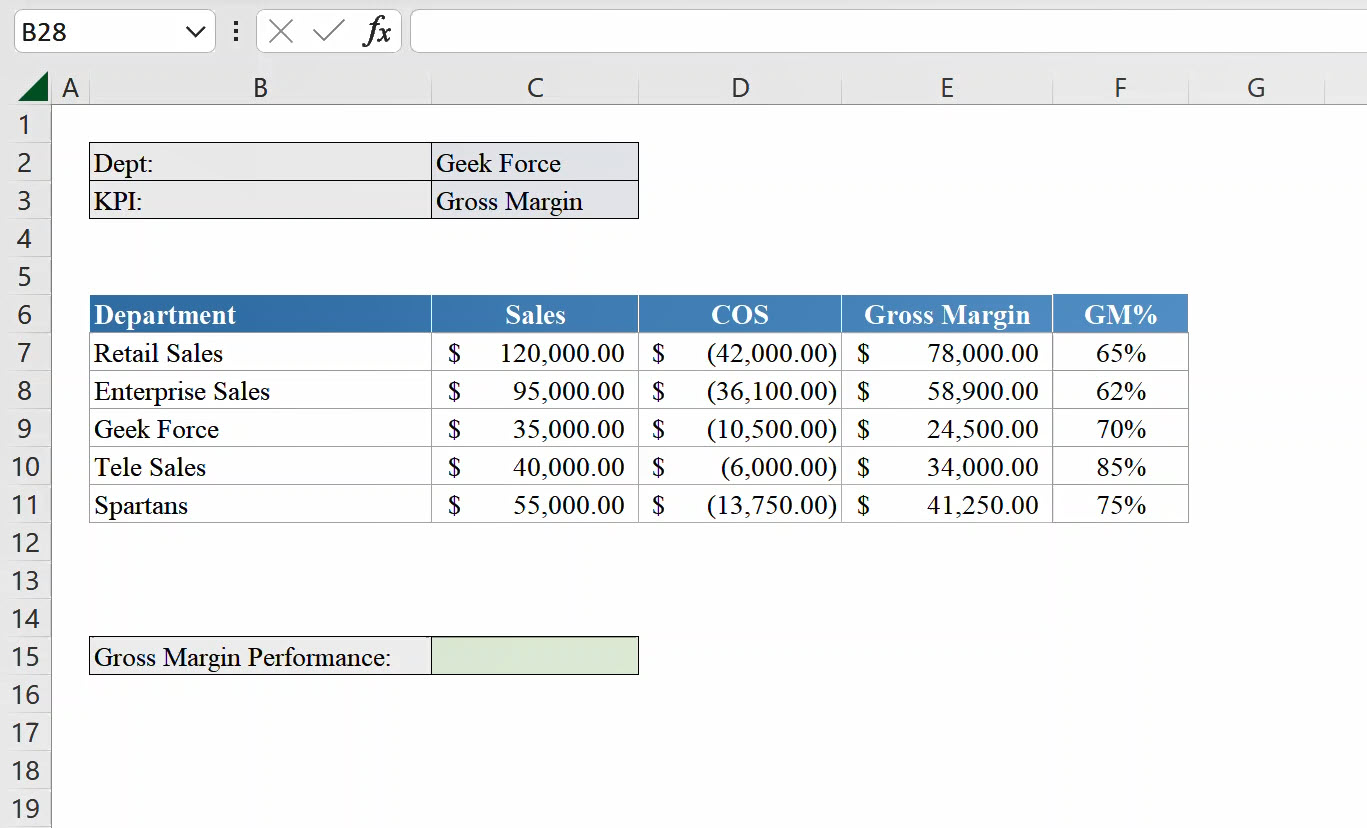
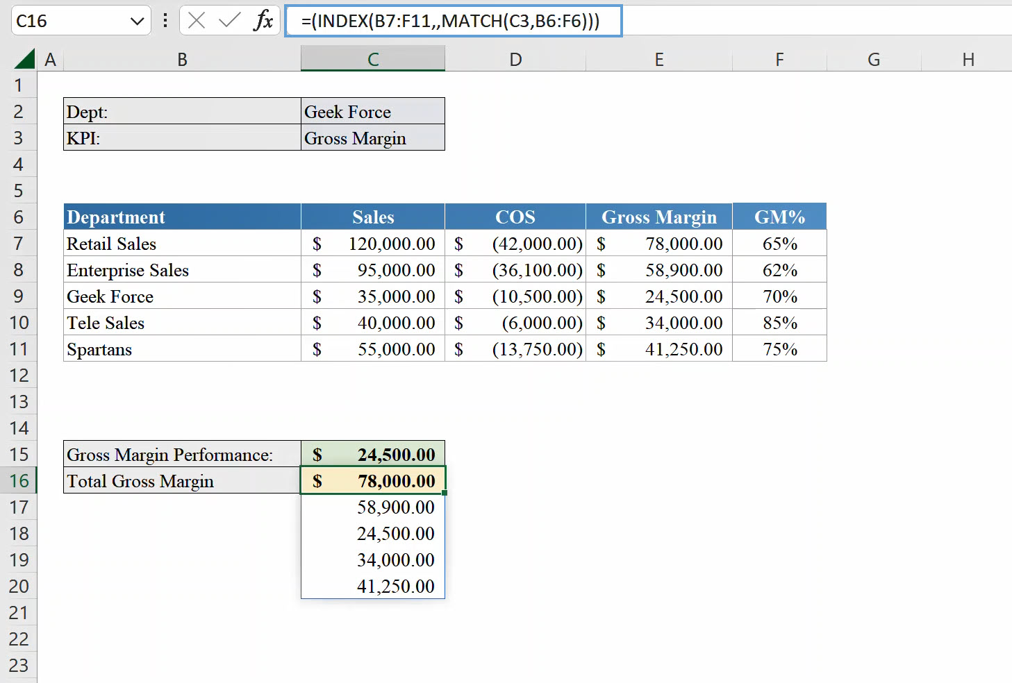
As you can see from the above, we need to retrieve the Gross Margin performance of the Geek Force. There are plenty ways to achieve this, but the easiest way is by using the INDEX & MATCH Combination. We would need to match both the row number and column number from our data set. Let's see the formula to use below:
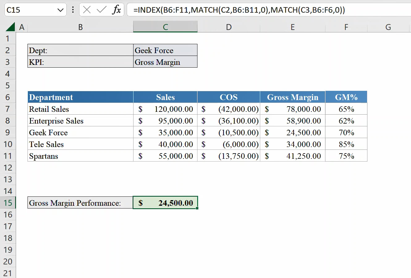
Now let's explain each part of the formula:
- INDEX(B6:F11: This represents the array argument. We selected the entire data set because we are going to specify both the row and column numbers.
- MATCH(C2,B6:B11,0): To automatically generate the row number based on the department chosen on C2 (Greek Force), we set the row number by using the MATCH function. Notice however that our match array is B6:B11, this is because the department names are on column B.
- MATCH(C3,B6:F6,0): Our second match function, this is used to automatically return the column number based on the KPI chosen. Our range for this is horizontal (B6:F6) because this is the heading where our KPIs are contained in.
Return all Values in a row or column
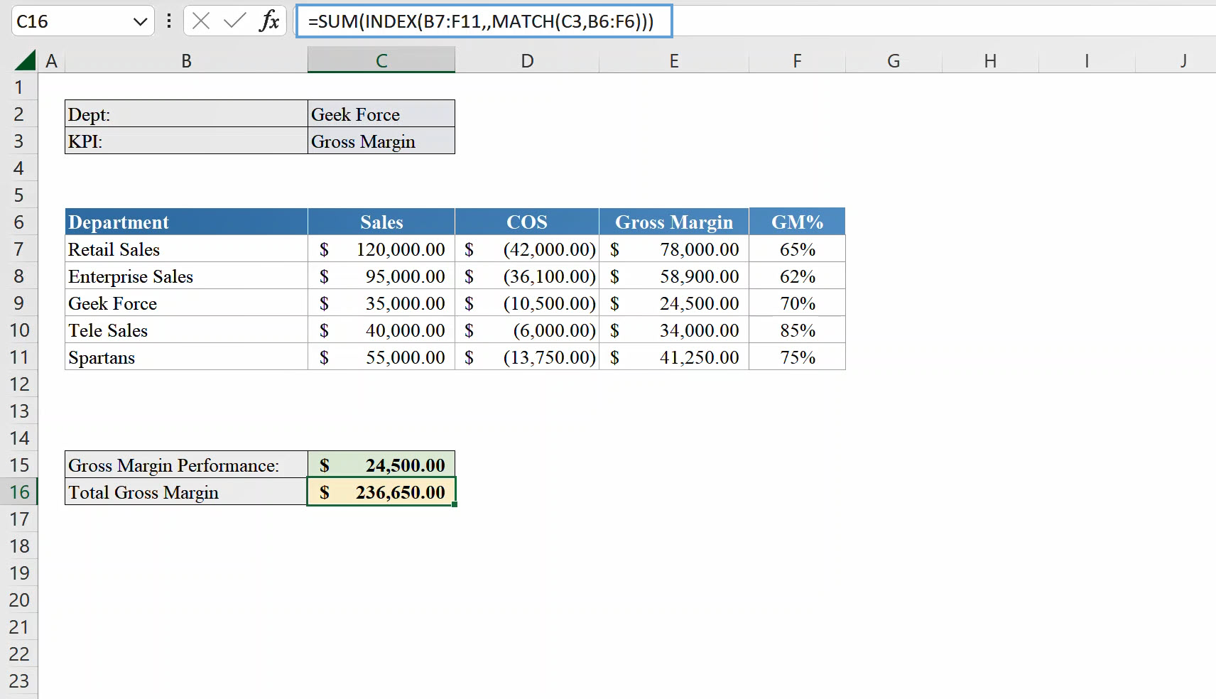
To return all values in a row or column, simply input any one of the row number or column number whilst leaving the other blank. Building on the previous example, let's assume we want to calculate the total value of the KPI we are currently evaluating (Gross Margin), we would only need to input the column number whilst leaving the row number blank. Formula to use is as follows:
The formula retrieves the entire range of Gross Margins, but we are interested in the sum of all Gross Margins. To achieve our target, we combine with a simple SUM function:
INDEX Function to create dynamic range in dropdown
With the Excel INDEX function, you can create a dynamic named range, we could then be used in a drop-down list. In this section, we would walk you through the steps for creating the dynamic named range and using it in your drop-down list. Let's begin shall we:
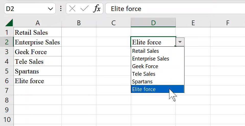
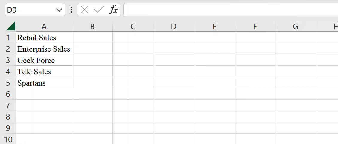
Let's extract the department name to a new worksheet and create a dynamic ranged drop-down list based on departments added to our column A as seen below:
To create the dynamic named range using the INDEX Function, please follow these steps:
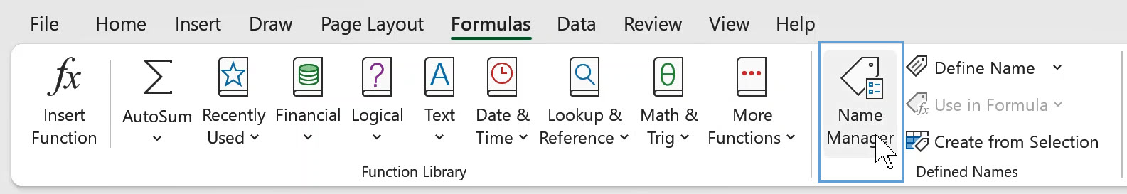
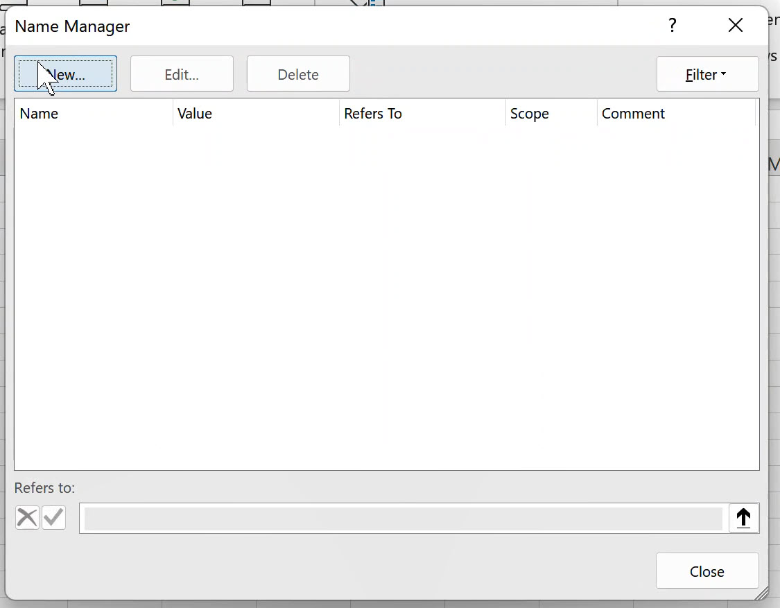
Step 1: Navigate to the Formula Tab and click on Name Manager
Step 2: Click on new in the name manager tab
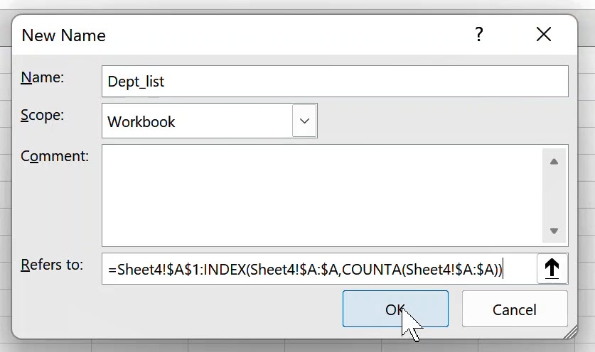
Step 3: Type in an easy to remember name in the "name" box and type in the formula below in the "Refers to" box and click on ok when you are done
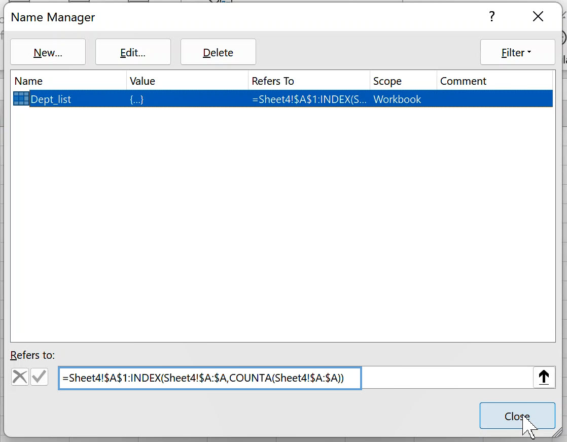
Result: A new named range would appear in the Name Manager:
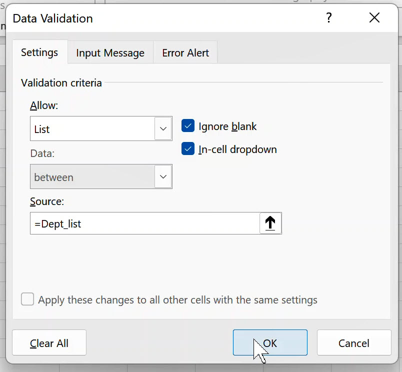
Now we are halfway there, all we need to do is to refer to the named range specified above in the Data Validation list. Navigate to the Data tab, and under the data group click on Data Validation.

Now click the drop down in "Allow:" and select List. For the Source, simply reference the Named range you created in the previous steps and click on OK
Result: We included a new department called Elite Force, let's see whether our drop-down captures this: