Table of Contents[Hide][Show]
In our INDEX Function post, we treated the INDEX MATCH Function combination, however that was for a single criteria lookup. In this post we would be reviewing how to combine the INDEX and MATCH Functions for an Index match multiple criteria lookup.
To Illustrate, we have prepared a data containing information on Merchandize Items my social enterprise is looking to sell for a fund drive to raise money for Indigent children's education:
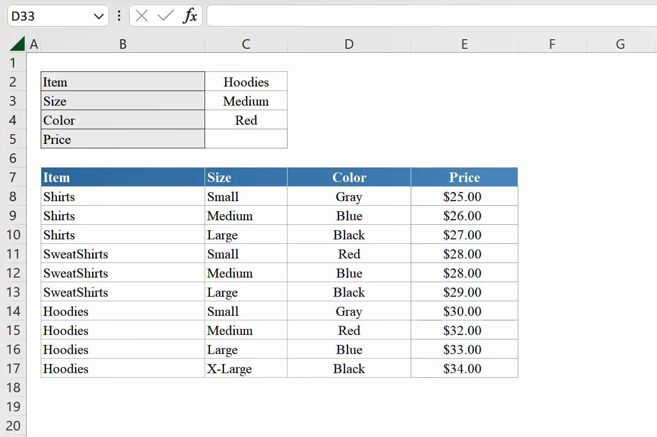
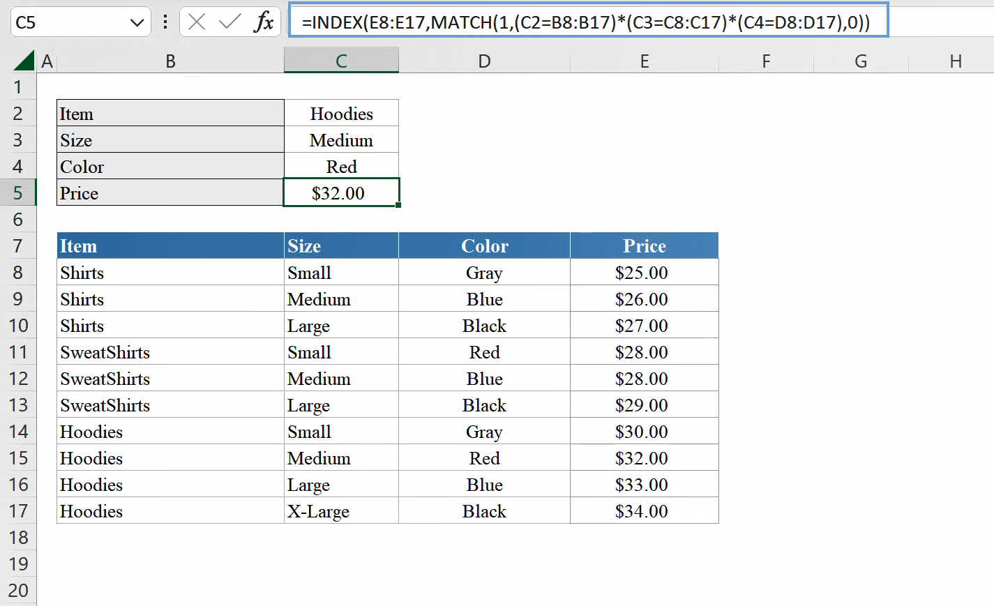
As you can see from the above, we need to return the price of an Item based on 3 criteria which are the Item name, the selected size and selected color. To achieve this, we use the formula below:
Explaining the Formula:
Our Index formula is really the standard Index formula with no column number input. On first view, it may look very complex, however it is really easy to remember once you understand how it works.
The first part of the formula "=INDEX(E8:E17" is the column for the price. Because we are not specifying the column number in this formula, we need to provide instruction regarding the single column the Function would pick from. If the range is a multi-column range such as E8:H17, the formula would return a #REF! error.
MATCH(1,(C2=B8:B17)*(C3=C8:C17)*(C4=D8:D17),0) calculates the row number and this is the key to retrieving the value for a multiple criteria INDEX MATCH lookup. You would see that the MATCH formula in this example is somewhat different from the usual formula. This is because we need to change the MATCH Function to an array formula and starting with 1 tells excel you have one or more criteria to confirm if true or false.
=INDEX(C:C,MATCH(1,B:B,0)) // Change to array Function by starting with 1
The next step would be to wrap each criteria after the "1," in brackets and connect with an asteriks operator (*). So each criteria would be (criteria1=range1)*(criteria2=range2)
For each criteria and range pair, excel would check each row in the range whether it is true that it matches the criteria and then move on to the next criteria and range pair. At the end of processing all the criteria and range pairs, excel matches rows that returned True, to get a single row that returned True for all logical tests.
{FALSE;FALSE;FALSE;FALSE;FALSE;FALSE;FALSE;TRUE;FALSE;FALSE}
{FALSE;FALSE;FALSE;TRUE;FALSE;FALSE;FALSE;TRUE;FALSE;FALSE}

Only the 8th entry for each row returns True for all cases, excel then calculates it to be the row number and then counts 8 down in the column you specified in the opening INDEX function: "=INDEX(E8:E17". The amount returned would be $32 based on meeting all criteria.

