When working with data sets with a lot of repetitive information, you may need to quickly identify the unique entries, this is where the remove duplicate button in excel comes in handy. In today's post, we would go through how to remove duplicates from a range in excel. Our focal point would include conditional formatting to identify duplicates and removing duplicates within a range.
Conditional Formatting to Identify Duplicates
Excel has built in conditional formatting that allows users format cells based on value and highlight duplicates, but this is done at cell level and not row levels. To achieve row level highlighting of duplicates, you would need a formula for that. We would walk you through both in this post. let's begin by evaluating the built in conditional formatting only, we would delve deeper into the advanced conditional formatting in later posts.
Excel Built In Highlight Duplicates
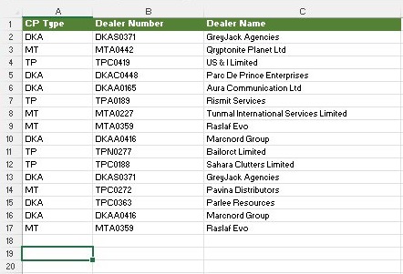
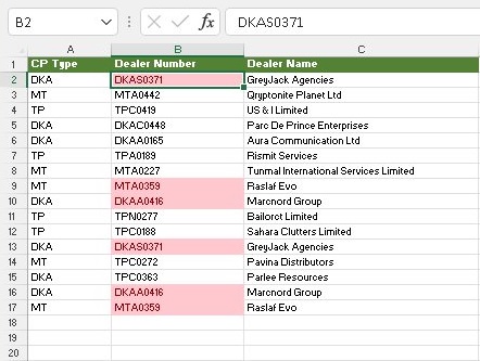
As already established, this works on cell level so it is best for identifying duplicates on a column by column basis. In today's example there are 3 columns that provide information on Channel Partners of a fictitious telecommunications company. Let's try to identify duplicates in the second column.
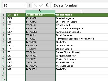
Step 1: Highlight the column you want to identify duplicates in by clicking on the column Letter as seen below.
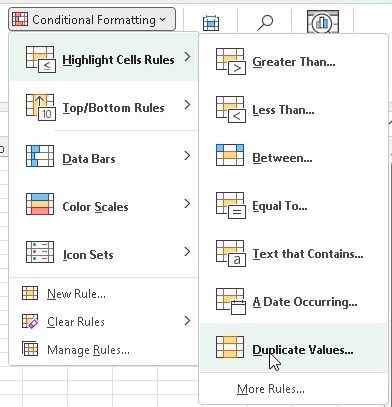
Step 2: On the home tab, click on Conditional Formatting > Highlight Cells > Duplicate Value
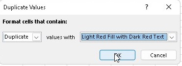
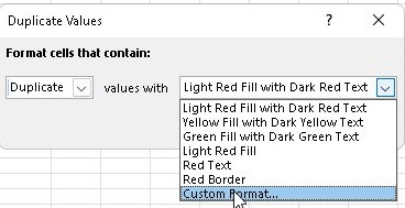
Step 3: In the selection box that pops out, you can go with the default format and click ok or use the drop down to select a custom format.
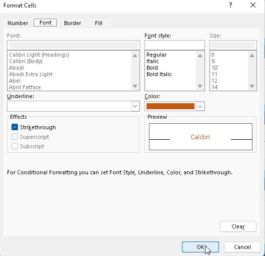
Or Format the duplicate cells by specifying your own font color, cell fill, border and so much more.
Result: All duplicate cells in column B are highlighted
Highlighting Duplicate Rows in Excel
To highlight duplicate rows in excel, just follow these simple steps:
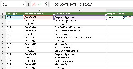
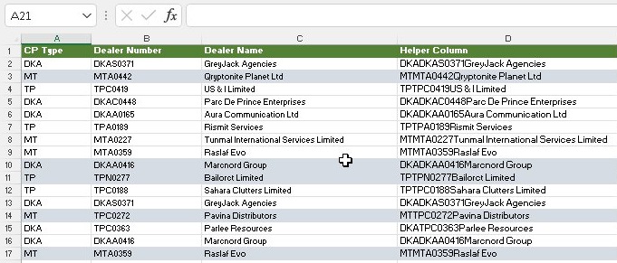
Step 1: Insert a column and combine previous columns on the same row by using Concatenate. This means that for every row in your data set, you should use the Concatenate formula to combine all preceding columns just like we did below.
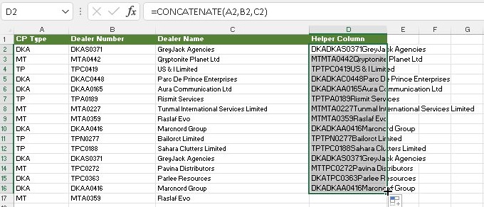
Step 2: Drag the formula to other rows in the dataset or copy and paste to the other rows or use Flash Fill
Step 3: Select the full range of the dataset (A1:D17)
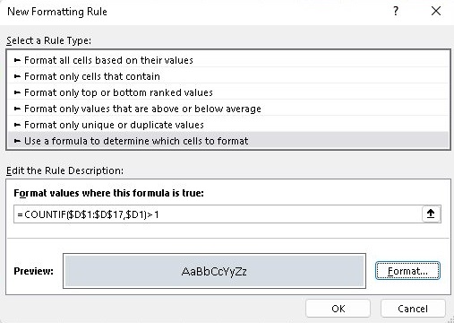
Step 4: Navigate to Home > Styles > Conditional Formatting and click on new rule.
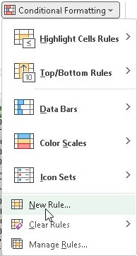
Step 5: Select "Use a formula to determine which cells to format", and type in this formula and click on ok: =COUNTIF($D$1:$D$17,$D1)>1
Result:
Removing Duplicates from a Range
Now that we have identified that there are duplicates in our dataset, how do we remove them? Easy, just follow these simple steps. Please note that you don't need to identify duplicates before removing them.
Step 1: Click on any cell within the dataset we worked on in the previous section.
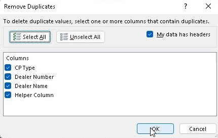
Step 2: Navigate to the data tab > data tools group, and click on remove duplicates

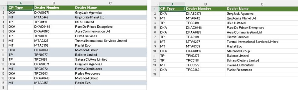
Step 3: Ensure that all checkboxes are checked and then click on ok
Result: You get a notification from excel about the number of duplicate values. Click on OK, and you should see your dataset without any duplicates. Excel removes all identical rows except for the first instance found (See the second image below)