Vlookup is one of the mot popular and most commonly used functions in excel. In this post, we would walk you through how to use the VLOOKUP excel function with easy-to-follow examples. Before we begin, let's review the purpose of using the VLOOKUP function.
Purpose of VLOOKUP Function
The VLOOKUP Excel function is used to lookup values from a data table organized vertically. It can look up approximate and exact matches, and you could even use it to look up wildcards (*?). The drawbacks of the Vlookup function however are that the lookup values must appear in the first column of the data table, and if there are two entries of the lookup value in the data table, the Vlookup function picks the first.
Syntax & Arguments
=VLOOKUP(lookup_value, table_array, column_index_num, [range_lookup])
- lookup_value: This is the value you are looking up in your data table, and as stated in the previous section, it must appear in the first column of the data table
- table_array: This represents the data table to retrieve a value
- column_index_num: This represents the column in the table to retrieve the data from
- [range_lookup]: With this, you specify whether you want an exact or approximate match. The default is True which represents approximate match, whilst False represents exact match. To avoid errors, it is most advisable that you set this to False to enforce exact match for your lookups.
Usage Notes
- The VLOOKUP Function can only search for the lookup value in the first column of the table array. If the lookup value is found in the table array, it can subsequently retrieve another value from columns to the right of the first column.
- The VLOOKUP function doesn't return values to the left of the first column in the table array. If you need to return values to the left of your lookup column (first column), please use the INDEX MATCH Functions combination.
- The function is case insensitive, it retrieves the value once the lookup value is found in the table array, regardless of the difference in cases between the lookup value and its match in the table array.
- If the Lookup value is not found, an N/A error is returned.
VLOOKUP Examples
We would be reviewing various examples to illustrate the use of the VLOOKUP function. Let's begin with VLOOKUP using the Exact match mode.
Exact Match Examples
In our example for this section, we have a data table of a few staff and their hourly wages, and to the right of the data table, we have section where we need to lookup the position and hourly wage of one of the employee IDs . Let's get to it shall we:
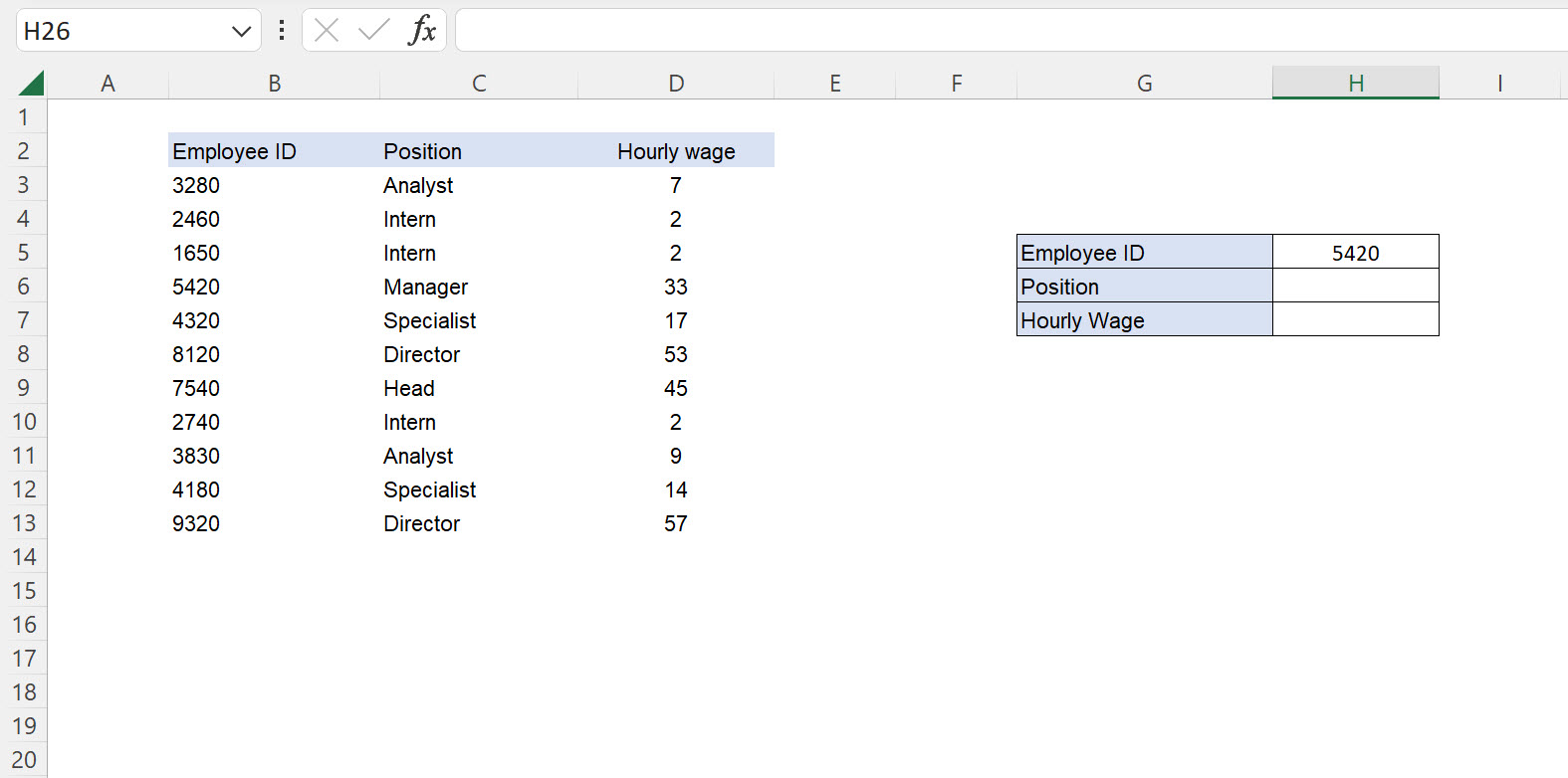
To return the Position of the Employee ID 5420, type the formula below in the section you have created for the lookup
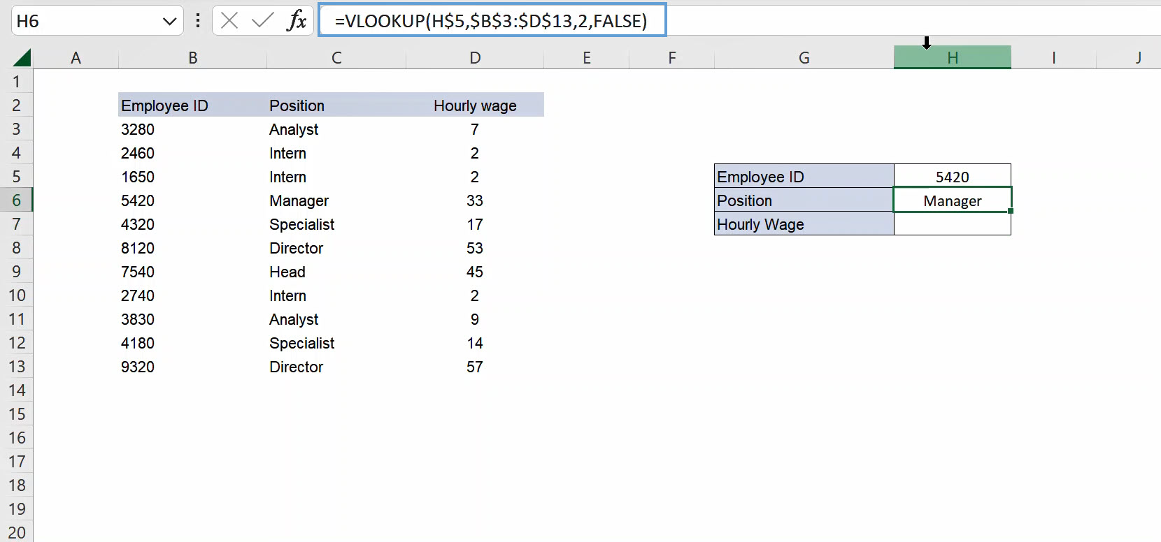
We have anchored the row (H5) of our lookup value by placing a dollar ($) sign right after the column letter whilst the anchored the entire table array B3:D13 by placing $ sign both before and after the column letter. The reason for doing this is to make it easier to copy and paste the formula in the cell we have prepared to lookup the hourly wage for the employee ID.
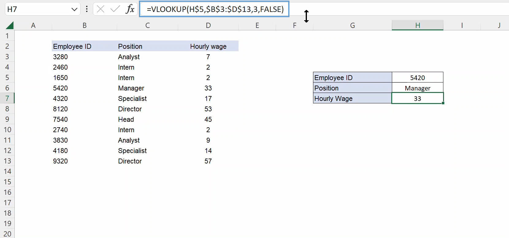
After pasting, all we need to do is to go into the formula and change the column number to 3 because it is 3 columns to the right of the employee ID in our data table. We say 3 columns because we count the Employee ID itself.
Now to lookup the hourly wage using the Vlookup function, use the formula below:
Approximate Match Examples
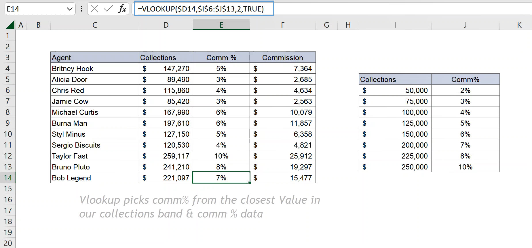
The VLOOKUP approximate match option is for when you desire the best match, but not necessarily the exact match. In our example for this section, VLOOKUP needs to be used in an approximate match mode because an exact match for our lookup value can't be found in our data set. Our example shows debt collections by agents and we need to apply a comm% based on the collections bands and comm% tox the right of the data set (Columns I:J)
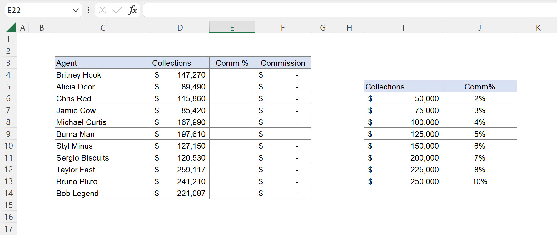
To apply the VLOOKUP by approximate match, select Cell E4 and use the formula below:

Copy and paste the formula to the other cells to return the results below:
Wildcard Match Examples
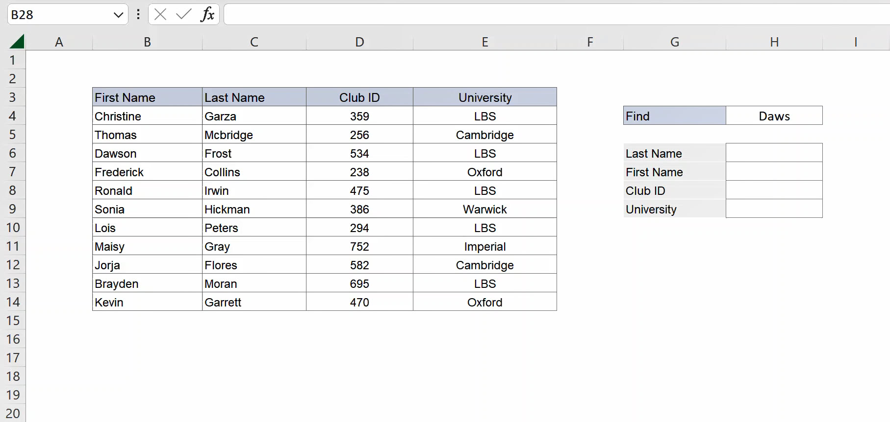
Wildcard Vlookup match enables you to lookup a partial match with (*). In this section, we have a data set containing information of a UK Inter-University club's leaders and our task is to lookup all details using Vlookup with Wildcards in our lookup section.
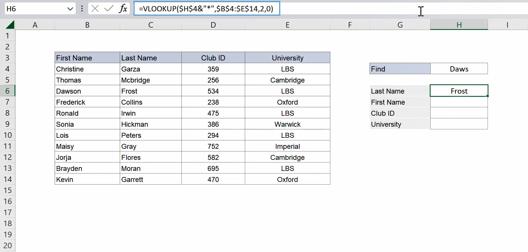
In our example above, we have been given a partial first name to lookup in cell G4. This would be impossible without the use of Vlookup WildCards. To use the Vlookup with wildcards, maintain the exact match (FALSE) lookup, however you would need to concatenate the cell containing the partial value and the * using the "&" operator. Please see the formula below:
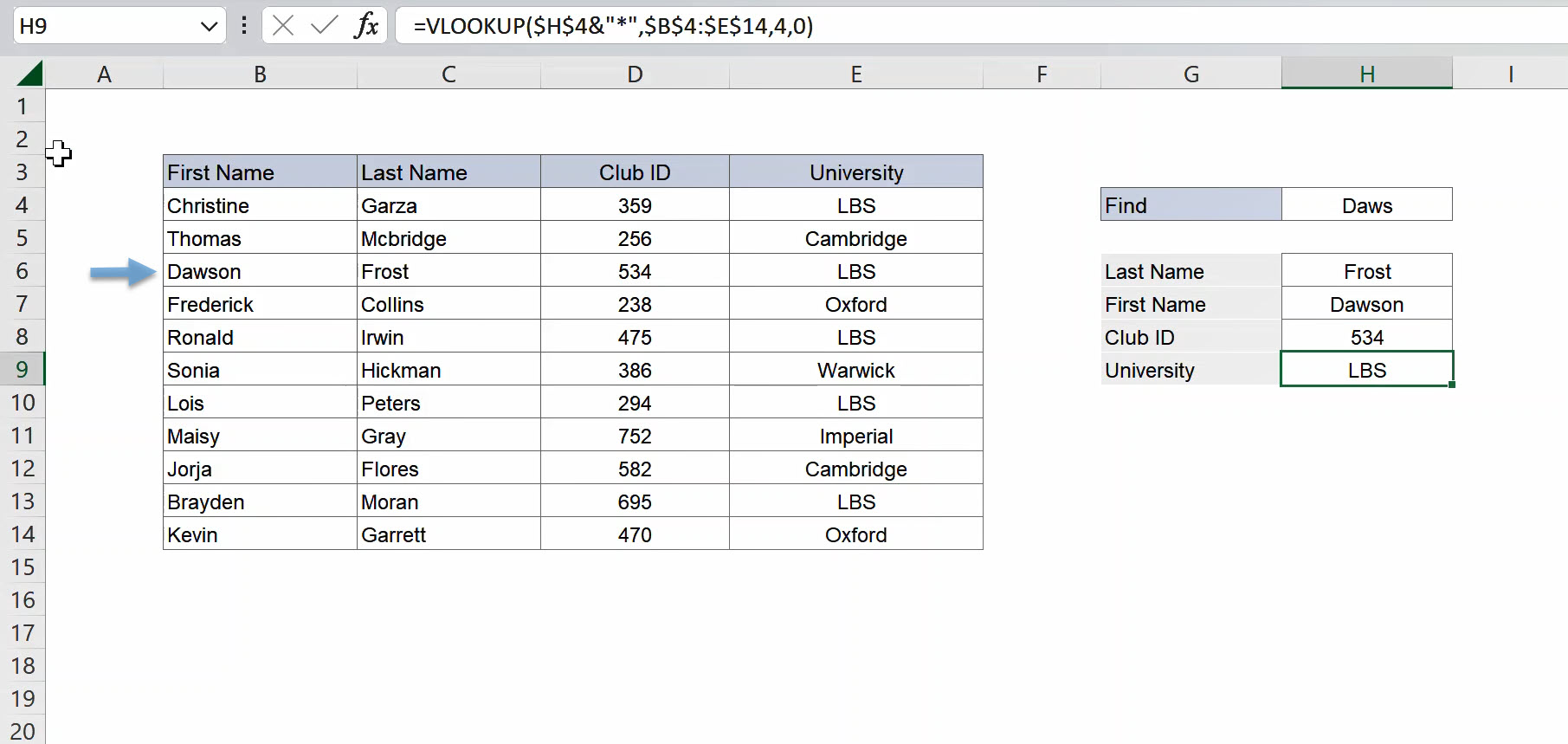
Now that we have gotten the first formula right, all we need to do is to change the column numbers as follows:
- Column 1: For First Name column, change ",2," in the formula to ",1,"
- Column 3: For Club ID, change ",2," in the formula to ",3,"
- Column 4: For University, change ",2," in the formula to ",4,"
If done correctly, you should have the following results:
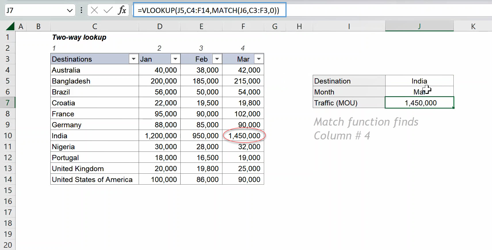
Two-Way Lookup
You would notice that the column number for the VLOOKUP function is usually hardcoded within the formula, you can change this by using a two-way lookup to locate the column number automatically. Confused? Don't worry, we would go through it in the paragraphs to come, however, let's briefly introduce you to our dataset for this section.
Our dataset is the traffic sent by users of a Mobile Network Operator (MNOs) to various destinations in the first quarter of the year. Our task is to lookup the traffic to a particular destination using a two-way lookup.

In our example, we need to find the traffic for India in the month of Mar. To achieve this, simply use the formula below to automatically match and calculate the column number for our Vlookup function: